A Simple Use of split(),cat(), print(), capture.output() Functions in R
  • split() splits a data in to many according to a function you provide
  • cat() means concatenate which pastes strings to concatenate the objects, and
  • capture.output() sends the output to the drive you specify in the format you specify
In one of my assignment in hydrological simulation, I had to present an output for 10 years that looked like the following and I used these functions to get my work done.
R is awesome; That's why I am Learning-R.

.
Oatka Creek - ABEN 678 - Prob. 3 - 1996 YEAR 2

PRECIP EVAPOTRANS GR.WAT.FLOW RUNOFF STREAMFLOW

-----------------(cm)----------------------------------

Apr 3.3 2.2 1.5 0.0 1.5

May 4.9 7.2 0.8 0.0 0.8

June 13.2 11.3 0.0 0.1 0.2

July 12.5 11.5 0.4 0.5 0.9

Aug 6.4 9.8 0.0 0.0 0.0

Sept 7.9 7.2 0.0 0.0 0.0

Oct 3.6 4.5 0.0 0.0 0.0

Nov 6.7 1.0 0.0 0.0 0.0

Dec 7.6 0.5 4.1 0.3 4.4

Jan 4.0 0.2 5.6 0.2 5.8

Feb 9.4 0.2 3.8 1.0 4.8

Mar 6.9 0.7 9.7 1.5 11.2

---------------------------------------------------------------

YEAR 86.4 56.4 26.0 3.6 29.6

Lets try to get such output using R.

I am going to start from the end of a simulation I did in R, the final codes of which looked like following. I had to write it to get the monthly and annual aggregates of the streamflow

library(zoo); library(chron)

Date<- seq(as.Date("1970-04-01"), as.Date("1980-03-31"), by = 1)

streamflow<- zoo(WATBAL, order.by = Date) ## WATBAL is an output file from the simulation

Lets create function to obtain annual and monthly sums

annual<- function(Date, result.file)as.integer(as.yearqtr(time(result.file))-0.25) This is because, I needed to start the year from April instead of January.
monthly<- function(Date, result.file) as.Date(as.yearmon(time(result.file)))
annual.flow<- aggregate(streamflow, annual(Date, streamflow), sum)
monthly.flow<- aggregate(streamflow, monthly(Date, streamflow), sum)
##This gives outputs like these
annual.flow
annual.flow
Ppt Et GwF Ro Sflow
1970 105.9 54.5 50.1 3.1 53.4
1971 86.2 53.5 25.6 3.5 29.2
1972 108.5 52.8 55.3 1.0 56.5
1973 103.9 56.5 48.3 2.2 50.7
1974 102.8 51.4 49.6 2.0 51.8
1975 106.5 56.1 46.2 5.5 51.7
1976 95.7 51.6 41.1 2.0 43.2
1977 133.8 54.2 68.3 10.4 78.5
1978 86.0 54.4 40.2 3.3 43.6
1979 100.4 53.9 45.3 2.9 48.2

monthly.flow
monthly.flow
Ppt Et GwF Ro Sflow
1970-04-01 3.5 2.4 1.1 0.0 1.1
1970-05-01 9.6 8.4 2.5 0.0 2.5
1970-06-01 7.7 11.1 0.1 0.0 0.1
1970-07-01 7.4 12.0 0.0 0.0 0.0
1970-08-01 15.7 10.1 0.0 1.4 1.4
1970-09-01 12.3 6.5 3.3 0.0 3.3
1970-10-01 14.2 3.9 5.6 0.2 5.8
1970-11-01 12.4 0.0 14.6 0.5 15.2
1970-12-01 3.5 0.0 5.6 0.0 5.6
1971-01-01 4.2 0.0 3.2 0.1 3.4
1971-02-01 10.5 0.0 5.7 0.8 6.5
1971-03-01 4.9 0.1 8.4 0.1 8.5
1971-04-01 3.3 2.0 1.5 0.0 1.5
1971-05-01 4.9 7.4 0.6 0.0 0.6
1971-06-01 13.2 11.6 0.0 0.1 0.1
1971-07-01 12.5 11.4 0.0 0.5 0.5
1971-08-01 6.4 9.5 0.0 0.0 0.0
1971-09-01 7.9 7.3 0.0 0.0 0.0
1971-10-01 3.6 4.3 0.0 0.0 0.0
1971-11-01 5.2 0.0 0.0 0.0 0.0
1971-12-01 6.4 0.0 4.3 0.3 4.6
1972-01-01 5.7 0.0 5.8 0.1 5.9
1972-02-01 6.1 0.0 3.9 1.0 4.9
1972-03-01 11.0 0.0 9.5 1.5 11.1
1972-04-01 9.0 2.1 7.6 0.0 7.7
1972-05-01 15.4 8.2 8.3 0.1 8.3
1972-06-01 14.8 9.7 2.4 0.3 2.7
1972-07-01 4.4 12.3 1.9 0.0 1.9
1972-08-01 7.7 9.2 0.0 0.0 0.0
.
.
.
.
.
Now I needed to combine those two file and get the output like the first one, for the whole simulation period
Here how I did using the cat() and print() function

mth<- rep(seq(1970:1979), each = 12)

Split the data;it should be a zoo object(a chronological object),as here data is handled according to the time)

mth.1<- split(monthly.flow, mth)
mth.no<- index(mth.1)
output<- function(mth.no, mth.1)
for ( i in 1: length(mth.no)){
cat("OATKA CREEK YEAR",i,'\n')
print(cbind(mth.1[[i]]))
cat("Total Flow",annual[[i]],annual[[i+10]],
annual[[i+20]],annual[[i+30]],annual[[i+40]], '\n\n')
}
output(mth.no,mth.1)

Now capture.output simply saves the output in to a file of your desire, I have tried .doc, .rtf. or .txt and it works
capture.output(output(mth.no, mth.1), file = "U:/HW3_monthly output.txt")

OATKA CREEK YEAR 1
Ppt Et GwF Ro Sflow
1970-04-01 3.5 2.4 1.1 0.0 1.1
1970-05-01 9.6 8.4 2.5 0.0 2.5
1970-06-01 7.7 11.1 0.1 0.0 0.1
1970-07-01 7.4 12.0 0.0 0.0 0.0
1970-08-01 15.7 10.1 0.0 1.4 1.4
1970-09-01 12.3 6.5 3.3 0.0 3.3
1970-10-01 14.2 3.9 5.6 0.2 5.8
1970-11-01 12.4 0.0 14.6 0.5 15.2
1970-12-01 3.5 0.0 5.6 0.0 5.6
1971-01-01 4.2 0.0 3.2 0.1 3.4
1971-02-01 10.5 0.0 5.7 0.8 6.5
1971-03-01 4.9 0.1 8.4 0.1 8.5
Total Flow 105.9 54.5 50.1 3.1 53.4

OATKA CREEK YEAR 2
Ppt Et GwF Ro Sflow
1971-04-01 3.3 2.0 1.5 0.0 1.5
1971-05-01 4.9 7.4 0.6 0.0 0.6
1971-06-01 13.2 11.6 0.0 0.1 0.1
1971-07-01 12.5 11.4 0.0 0.5 0.5
1971-08-01 6.4 9.5 0.0 0.0 0.0
1971-09-01 7.9 7.3 0.0 0.0 0.0
1971-10-01 3.6 4.3 0.0 0.0 0.0
1971-11-01 5.2 0.0 0.0 0.0 0.0
1971-12-01 6.4 0.0 4.3 0.3 4.6
1972-01-01 5.7 0.0 5.8 0.1 5.9
1972-02-01 6.1 0.0 3.9 1.0 4.9
1972-03-01 11.0 0.0 9.5 1.5 11.1
Total Flow 86.2 53.5 25.6 3.5 29.


Multiple variables in the same scatter plot

HELLO,
Here, is another simple but very cool grapch R can create quickly. I find it the easiest way to create scatter plots especailly when I have to present two dependent variables with only one x-variable. I think this is not easily obtained EXCEL which we mostly use to obtain quick plots. But grahics is R's another speciality.
Here is how we can make a scatter plot with two dependent variables in it.

#Lets create the variables first. I am adding some noise to both dependent variable to make the plot look pretier.

x<-1:100
y<-x + sqrt(sample(x))
z<-x - sqrt(sample(x))

#plot x vs y

plot(x,y, col = 'blue',pch = 16,xlab = 'x', ylab = 'y,z')

#Now to add the plot of x vs z in the same graph,

points(x,z, col = 'red', pch = 16)

The output will look like this

But this picture doesn't tell us which is y and which is z. But we can easily add a legend to this with legend() command

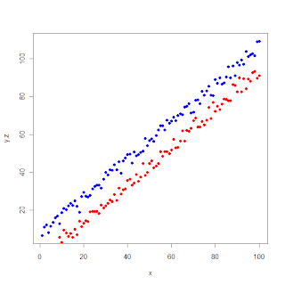
legend(10,85,legend = c("y","z"), col = c("blue", "red"),pch = 16)

# here 10, and 85 are the xy-coordinates where the legend-box will be added on the graph.


Now the graph is complete
.


Isn't this easy and quick? That's why I am a fan of it.


Article about R in NYTimes


I was just browsing the net and found an interesting and very good article in NYtimes.

I am touched by the first sentence. R could be just 18th letter of English alphabet ………………., that’s exactly what happened many times when I mentioned R in some friends circle.

Data accessing, editing and Manipulation


lets create some vectors,

   1: Var1<-c(1,2,3,1,2,4,5,0,2,6,8,5,3,7,5,2,8,9,2,10)
   2: Var2<-rep(c(1,2,3,4) each=5)
   3: Var3<-rep(1:5, 4)

now, lets make a data frame


   1: > datalist<-data.frame(Var1, Var2, Var3)


   Var1 Var2 Var3
1     1    1    1
2     2    1    2
3     3    1    3
4     1    1    4
5     2    1    5
6     4    2    1
7     5    2    2
8     0    2    3
9     2    2    4
10    6    2    5
11    8    3    1
12    5    3    2
13    3    3    3
14    7    3    4
15    5    3    5
16    2    4    1
17    8    4    2
18    9    4    3
19    2    4    4
20   10    4    5

so, the variable names can be changed now with,


> names(datalist)<-c("X", "Y", "Z")

Data Access:


> datalist[1:4,]


  X Y Z
1 1 1 1
2 2 1 2
3 3 1 3
4 1 1 4


> datalist[1:3,1:3]


  X Y Z
1 1 1 1
2 2 1 2
3 3 1 3


> datalist[3,3]


[1] 3


> datalist$X[c(2,5,8)]

[1] 2 2 0


> datalist$X[-c(2,5,8)]

[1]  1  3  1  4  5  2  6  8  5  3  7  5  2  8  9  2 10


> datalist[c(2,5,8),c(1,2)]

  X Y
2 2 1
5 2 1
8 0 2


Note that, X variable can not be accessed directly and we used datalist$X , if we want to access X directly we can use attach() function


> X
Error: object "X" not found
> attach(datalist)
> X
 [1]  1  2  3  1  2  4  5  0  2  6  8  5  3  7  5  2  8  9  2 10

Generating treatment maps for a typical CRD experiment

Hellooo! 

For the last couple of weeks, I have been learning to write some R functions for simple biological systems simulations. Well, I haven't been that successful in that venture, but I surely learned some pretty useful things that we can do in  R w/o spending much time and brain.

Generating  the plot map in a completely randomized desine.

I think experimental designs are the inextricably related with most agricultural studies.  So, at least for me, knowing this code will make my work a bit easier in future.

Here is a code that generates a randomized treatment map for a CRD experiment

> no.treat<- ntrt<- 6
> no.repln<- nrepl<- 4
> trt.samples<- sample(rep(x = 1:no.treat, times = no.repln))
# This will generate random sampls for all the 6 treatments and repeat this for all the 6 replications.
> trt.map<- matrix(trt.samples, nrow = no.repln, ncol = no.treat)
# This will create a matrix of the random samples which is also the plot map of the experiment.
which looks like as follows
> trt.map
     [,1] [,2] [,3] [,4] [,5] [,6]
[1,]    5    1    6    6    5    3
[2,]    2    3    6    2    4    4
[3,]    4    3    2    1    2    5
[4,]    4    1    6    5    1    3
This is pretty easy, isn't it.